By Suraj Gupta in RStats — Mar 29, 2012

How R Searches and Finds Stuff

Or…

How to push oneself down the rabbit hole of environments, namespaces, exports, imports, frames, enclosures, parents, and function evaluation.

Motivation

There are a few reasons to bother reading this post:

Rabbit hole avoidance
You have avoided the above mentioned topics thus far, but now it’s time to dive in. Unfortunately you speak English, unlike the R help manuals which speak “Hairy C” (imagine a somewhat hairy native C coder from the 80s who’s really smart but grunts a lot…not the best communicator).
R is acting a fool
Your function used to work, now it spits an error. Absolutely nothing about this particular function has changed. You vaguely remember installing a new package, but what does that matter? Unfortunately my friend, it does matter.
R is finding the wrong thing
You attached the matlab package and call sum() on a numeric matrix. The result is a vector of column sums, not a length 1 numeric. This messes up everything. What were you thinking trying to make R act like Matlab? Matlab is for losers (and rich people).
You want R to find something else
You like a package’s plotting function. If you could intercept one call within the function and use your own calculation, it would be perfect. This seems like black magic to you, but something is strange about maintaining a full copy of the function just to apply your little tweak. Welcome to the dark arts.
Package authoring
You have authored a package. How does your kid plays with the other kids in the playground?

Where does R put things?

Everything is R lives in an environment. Ultimately, we’re trying to figure out which environment something lives in, and how we get there (or how we got there). An environment, like everything else in R is an object. Objects hold stuff. Environments are specialized, they can only hold two things:

A frame
This is just a collection of named objects. What’s a named object? Everything in R is an object, so it can be a function, a numeric, a character, a logical, etc. And these objects have names like myFunction, myNumeric , myCharacter, myLogical. When you type myVar = "charlie" at the command prompt you create a character object that holds the string "charlie" and you’re calling that object myVar. Since everything in R lives in an environment and the frame is the place where an environment holds objects, then the object you just created called myVar lives in a frame within some environment.
The environment’s owner aka the enclosing environment.
This is just a reference to another environment.

As you can see from the visualization above, the chain of enclosing environments stops at a special environment called the Empty Environment. You can access this object by executing emptyenv() in R. And given an environment object, you can query the object for the two things that matter: the environment’s owner and the objects in the frame.

A Fib About Owners and Pointers

Before you hit send on that flame mail I acknowledge a technical misdirection that I have and will continue to make. I use the concepts of ownership and containment loosely. I will say own or contain when I really mean pointer. If pointer means nothing to you then skip to the next section.

I will continue to talk about environments as owning objects, particularly functions. In truth functions are instructions stored somewhere in memory, and they are accessed by symbols in lookup tables that, when found, give a pointer to them. The core concepts of this article are agnostic to pointers and understanding pointers is unnecessary to achieve mastery of the search mechanism in R. In fact, R tries really hard to hide pointers. So yes it pains me to be technically imprecise, but I’m trying to keep things simple because most people can understand an ownership relationship and we have a lot of ground to cover.

Play time with Environments (don’t skip me)

# environments are just objects.  let's create one.
> myEnvironment = new.env() 

# print it out...
> myEnvironment 
<environment: 0x0000000006ce0920>

# every environment (except R_EmptyEnv) has an enclosure.
# Who's myEnvironment's enclosure?  It's "R_GlobalEnv" - find out using parent.env()
> parent.env( myEnvironment ) 
<environment: R_GlobalEnv>

# Who's R_GlobalEnv's enclosing environment? 
# It's the environment called "package:stats" (in my installation, might be different on yours)
> parent.env( parent.env( myEnvironment ) ) 
<environment: package:stats>
attr(,"name")
[1] "package:stats"
attr(,"path")
[1] "C:/R/R-2.14.1/library/stats"

# Here's two other ways to ask the same question. 
# This R_GlobalEnv must be special if it can retrieved using the identifier
# .GlobalEnv AND a function globalenv().  We'll discuss R_GlobalEnv later.
> parent.env( .GlobalEnv ) 
<environment: package:stats>
attr(,"name")
[1] "package:stats"
attr(,"path")
[1] "C:/R/R-2.14.1/library/stats"
> parent.env( globalenv() )
<environment: package:stats>
attr(,"name")
[1] "package:stats"
attr(,"path")
[1] "C:/R/R-2.14.1/library/stats"

# The empty environment is accessed using emptyenv() 
> emptyenv()
<environment: R_EmptyEnv>

# Why does myEnvironment have a funky name 0x0000000006ce0920? 
# That's just the location of the environment in memory.
# We can add a friendly name by assigning a "name" attribute.
# Unfortunately R doesn't replace the funky name with the friendly name when printing.
# We can use the environmentName() function to verify our cool name 
> attr( myEnvironment , "name" ) = "Cool Name" 
> myEnvironment 
<environment: 0x0000000006ce0920>
attr(,"name")
[1] "Cool Name"
> environmentName( myEnvironment ) 
[1] "Cool Name"

# let's create a numeric object
> myValue = 5

# Unless you try hard, when you create an object it is automatically placed in the 
# "current" or "local" environment, accessible using environment()
> environment() 
<environment: R_GlobalEnv>

# And we can query an environment for all objects in the frame using ls().
# Here we verify that objects myEnvironment and myValue
# are both placed in the local environment, R_GlobalEnv
ls( envir = environment() )
[1] "myEnvironment" "myValue"      

# We can override the default behavior and create an object
# in an environment other than the local environment.  
# To do this use the assign() function.  Here we create variable "myLogical" inside myEnvironment.
# We use ls() to verify that there was nothing in myEnvironment before the assignment, 
# and again ls() verifies that "myLogical" is inside myEnvironment after the assignment
> ls( envir = myEnvironment )
character(0)
> assign( "myLogical" , c( FALSE , TRUE ) , envir = myEnvironment )
> ls( envir = myEnvironment )
[1] "myLogical"

# We can retrieve any named object from any given environment using the get() function
> get( "myLogical" , envir = myEnvironment )
[1] FALSE  TRUE

# How could I have known that myEnvironment's enclosure would be R_GlobalEnv
# before I created the object? 
# Once again, R uses the local environment as the default value.  
# You can change an environment's enclosure using the replacement form of parent.env().
> myEnvironment2 = new.env()
> parent.env( myEnvironment2 )
<environment: R_GlobalEnv>
> parent.env( myEnvironment2 ) = myEnvironment
> parent.env( myEnvironment2 )
<environment: 0x0000000006ce0920>
attr(,"name")
[1] "Cool Name"

# Here's another way to understand the "current" or "local" environment
# We create a function that calls environment() to query for the local environment. 
# When R executes a function it automatically creates a new environment for that function.
# This is useful - variables/objects created inside the function
# will live in the new local environment.
# We call Test() to verify this.  We can see that Test() does NOT print R_GlobalEnv. 
# We didn't created any objects within Test().  If we had, they would live in the "0x0000000006ce9b58"
# environment while Test() is running.  When the function completes executing, the environment dies.
> Test = function() { print( environment() ) } 
> environment()
<environment: R_GlobalEnv>
> Test() 
<environment: 0x0000000006ce9b58>

# And why not...who's the enclosing environment?
# There's more than meets the eye here.  We'll go deeper in a bit...
> Test = function() { print( parent.env( environment() ) ) }
> Test()
<environment: R_GlobalEnv>

Short Answer: How R Searches and Finds stuff

Have you followed along with the code above? It seems that environments are not just static repositories of objects. When R executes an expression, there is always one local or current environment. Maybe it's easier to think of this as the active environment, in contrast to the other environments which are inactive. Or perhaps it's more intuitive to think of an expression executing “within” a particular environment. The point here is that at any moment R can ask “hey, what’s the local environment.” R asks this questions a lot. In fact, it asks this question every time it needs to find a named object. We saw that R creates a new local environments every time it runs a function. So when we run any decently involved piece of code, functions call other function and environments spawn and die.

Imagine we just freeze the system at any one expression. When R goes searching for the names in that expression, it first looks at the objects within the local environment. If the object is not found by name in that environment, then R searches the enclosing environment of the local environment. If the object is not in the enclosure, then R searches the enclosure’s enclosure, and so on. That’s how R searches and finds stuff; it traverses the enclosing environments and stops at the first environment that contains the named object.

Satisfied? I didn’t think so. Let's roll…

Map of the World (follow the purple line road)

We just said that R searches through the chain of enclosing environments to find named objects. It's sort of like a treasure hunt that is limited to a single direction. What we need for this treasure hunt is a map of the world!

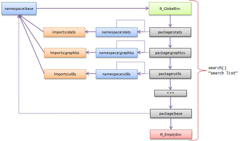
This graphic shows the state of all environments when you first startup R. Each box represents a unique environment. The solid purple line represents the enclosing environment relationship. I’ll explain the dotted purple line in a bit. For now, consider it a relationship that’s similar to the enclosing environment.

The Global Environment

I said that R_GlobalEnv is a special environment and you can see that it is colored green in the map. Green means start. The global environment is precisely the environment that you start at when you launch R. It is your current or local environment when R launches. If you make an assignment at the prompt, the named object is stored in R_GlobalEnv.

# the ls() function shows us all objects defined in a given environment.
# In this case we're using the identifier .GlobalEnv to refer to the global environment
# Here we can see that upon startup the global environment contains no objects
# but after we assign myVariable, the global environment contains an object with that name
> ls( envir = .GlobalEnv ) 
character(0)
> myVariable = 0 
> ls( envir = .GlobalEnv )
[1] "myVariable"

# be careful with the environment() function.  It might seem wrong that this returns NULL
# but if you read the documentation you'll see that environment() takes a function as input.
# myVariable is not a function, it's a numeric.  The purpose of environment() is not to tell you
# an object's owner.  More to come...
> environment( myVariable )

The Search List

In R, the “search list” is the chain of enclosing environments starting with R_GlobalEnv and ending with R_EmptyEnv. I like to think of it as the main highway on our map. This is the highway that R drives down when we start in R_GlobalEnv. All roads in our world eventually lead to this highway. You can obtain the search list by typing search() at the prompt:

> search() 
[1] ".GlobalEnv"        "package:stats"   "package:graphics" "package:utils" "package:datasets" 
[6] "package:grDevices" "package:methods" "Autoloads"        "package:base"

Package v. Namespace v. Imports Environments

If you stare at our map above for enough time you might notice that every R package has 3 associated environments. If you think that this is confusing then you are blessed with common sense. This drove me crazy when I first encountered it. Trust me for now that the only tricky part about this is the naming convention, otherwise this trifecta is useful and well-designed.

Here’s a breakdown, left to right:

package environment
This is where a package’s exported objects go. Simply put, these are the objects that the package author wants you to see. These are most likely functions. Typically a package is published that provides useful functions related to some topic or domain. In traditional Object Oriented Programming (OOP), this is analogous to a “public” class or method. If that means nothing to do you then ignore it.
namespace environment
This is where all objects in a package go. This includes objects the package author wants you see. It also includes objects that are not meant to be accessed by the end-user. The latter, the “hidden” objects (they are not really hidden, you can access them if you’d like) facilitate the “visible” ones. For example, a function HardCalculation() might offload some complicated text formatting tasks to function MakeResultsPretty(). The author doesn’t want you to call MakeResultsPretty(), its sole purpose is to format the results that are idiosyncratic to HardCalculation(). In OOP this is analogous to a “private” or “internal” class or method. You might be thinking “wait, so objects the author wants me to see are in BOTH the package environment and the namespace environment?” Yes and No. Yes, both environments have a frame that lists objects of the same name, but no there is not two copies. Both environments have pointers to the same function. If that makes no sense to you then think of it as two copies - it honestly doesn’t matter. This may seem like an odd arrangement (two pointers, two copies - your pick) but its use will become apparent shortly. This is also why there is no easy way to query an object for the environment that owns it. It's possible that two or more environments own the same object.
imports environment
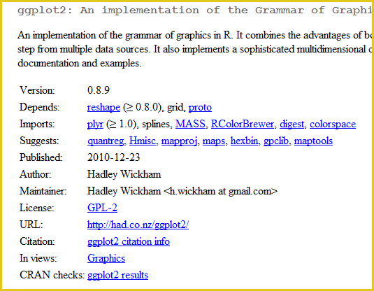
This environment contains objects from other packages that are explicitly stated requirements for a package to work properly. Most packages published on CRAN are not islands; they build on functionality provided in other packages. Take ggplot2 for example. You can see on the CRAN page in the “Imports” section that it requires plyr among other packages. I suggest using the screenshot below since the package could change in a way that breaks my example. The imports:ggplot2 environment contains all objects in the plyr package.

Imports v Depends

You might have been confused seeing a Depends and an Imports section. If Imports states a package’s requirements, then what does Depends do? This is a poor naming convention. The Depends section also lists packages that ggplot2 requires. The difference between Imports and Depends is where the requirement is placed on our map of the world. Because our map specifies the path R takes to find objects, there are consequences to specifying a requirement in Imports versus Depends in terms of how R finds the dependency.

If the package is specified in Imports, then the package contents will go into the “imports” environment. In the case of ggplot2, the objects in the plyr package will appear in the imports:ggplot2 environment. Notice also that plyr does not have a package environment. It's nicely tucked away inside the environment imports:ggplot2. The dotted purple line will be explained later.

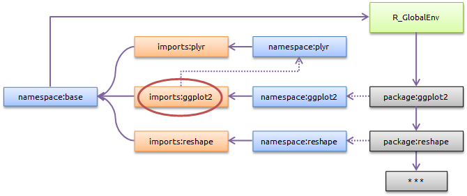
If a package is specified in Depends (i.e. reshape package), then the package is loaded as it would be if you called library() or require() from the R prompt. That is, the package, namespace, and imports environments are created for the dependency and placed on our map. The reshape package is attached before ggplot2 and the package:reshape environment becomes package:ggplot2’s enclosing environment.

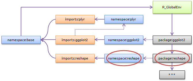
So who cares? Is the choice between Depends and Imports arbitrary? It's not. The library() command (or generally attaching a library) places the package environment under R_Global. More precisely, the package environment becomes R_Global’s enclosing environment. R_Global’s old enclosure now encloses the package environment. You can see this in the diagram below where we have loaded the package reshape2 which is a re-write/upgrade of the original reshape package.

Both reshape and reshape2 contain the function cast. Let's say (I’m making this up) that ggplot2 has a function called FunctionThatCallsCast(). As you can guess, this function calls the cast() function. Without knowing any details of how R finds stuff, let's just follow the “purple line road”. We travel from to 1 and 2 and find FunctionThatCallsCast(). Remember, the package and namespace environments both reference a package’s public-facing functions. We execute that function and now we need to find cast. We travel from 3 to 5 searching for cast. We find cast at 6 and stop. But this is the wrong cast. This is cast in package reshape2, but ggplot depends on the cast in reshape. This could have dire consequences depending on the differences between cast in reshape and reshape2.

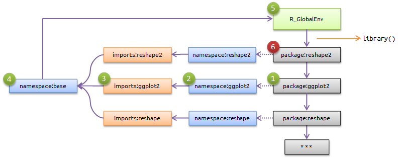
The better solution would have been to stuff reshape’s cast() function into imports:ggplot2 using the Imports feature. In that case, we would have travelled from 2 to 3 and stopped. Now you can see why the choice between Imports and Depends is not arbitrary. With so many packages on CRAN and so many of us working in related disciplines it's no surprise that same-named functions appear in multiple packages. Depends is less safe. Depends makes a package vulnerable to whatever other packages are loaded by the user.

namespace:base

We haven’t mentioned the fact that all imports:<name> environments have namespace:base as their enclosure. Think of this a freebie for creating a package. Since the base functions are used frequently, they are most likely a dependency for any package (or a package’s imports). Without namespace:base where it is, R would have to go hunting quite far to find package:base. There’s a big risk that another package has a function of the same name as a base function. A package author cannot know a-prior when you intend to attach her package nor that you have decided to write your own version of a base function. So do as you like, a package author can expect that R will find the base functions immediately after Imports. There’s no chance of corruption.

The Curveball (the dotted purple lines)

Functions, like all objects, are housed inside environments. However, functions themselves have a property which is a pointer to the environment in which they should run. When you create a function, that property is automatically set to the environment in which the function was created. So the environment that houses a function and the environment that the function will run in is one and the same.

What do we mean by “the environment that a function will run in?” We said earlier that executing a function creates a new environment specifically for that function. We also said that all environments have an enclosing environment. So what environment is the enclosure of the function’s new environment? This is what is specified by the function’s environment property. This is “the environment that a function will run in.” It's not necessarily the environment that owns the function. It is controlled by the function’s environment property.

We can get a function object’s environment property using the environment() function. For example:

> MyFunction = function() {} 
> environment( MyFunction ) 
<environment: R_GlobalEnv>

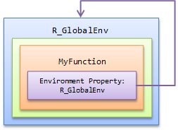
And when we run MyFunction() and R is executing lines of codes inside that function, the environments look like this:

By default, R sets a function’s environment property equal to the environment where the function was created (the environment that owns the function). However, it's not necessary that a function’s executing environment and the environment that owns the function are one and the same. In fact, we can change the environment to our liking:

# notice how environment(MyFunction) no longer returns R_GlobalEnv
> MyFunction = function() { } 
> newEnvironment = new.env() 
> environment( MyFunction ) = newEnvironment 
> environment( MyFunction ) 
<environment: 0x000000000e895628>

# Another way to see a function's environment property is to just print 
# the function. The environment will appear at the bottom of the printed function 
> MyFunction
function() { } 
<environment: 0x000000000e895628>

# Here we do the same for the standard deviation function
> environment( sd ) 
<environment: namespace:stats> 
> sd 
function (x, na.rm = FALSE) 
{ 
  ... (removed for brevity) 
} 
<bytecode: 000000000E7F2EA0>
<environment: namespace:stats>

# Can you figure out what's going on here? 
# When run, FromLocal's enclosing environment is the MyFunction environment.  That's where 
# FromLocal was created and that's what R does by default.
# When R searches for the object "age" within FromLocal it looks to the MyFunction environment,
# picks-up age = 22 and adds 1 to that. 
# -
# When run, FromGlobal's enclosing environment is R_GlobalEnv because 
# we assigned the function's environment property to R_GlobalEnv.
# When R searches for "age" within FromGlobal, it looks at the enclosing environment which is 
# The Global environment, and picks up age = 32 and adds 1 to that.  
# -
# The environment of NoSearch() already has 
# the age object and does not need to search its enclosing environment(s).
> age = 32 
> MyFunction = function() 
+ { 
+     age = 22 
+     FromLocal = function() { print( age + 1 ) } 
+     FromGlobal = function() { print( age + 1 ) } 
+     NoSearch =  function() { age = 11; print( age + 1 ) } 
+     environment( FromGlobal ) = .GlobalEnv 
+     FromLocal() 
+     FromGlobal() 
+     NoSearch() 
+ } 
> MyFunction() 
[1] 23 
[1] 33 
[1] 12

This explains the dotted purple lines in our map. If you inspect the environment property of the functions within the package:<name> environments you’ll see that they all point to the namespace:<name> environment. Check it out:

# get the standard deviation function within package:stats and
# inspect the function's environment property.
# Notice that it points to the namespace:stats environment
> statsPackageEnv = as.environment( "package:stats" ) 
> sdFunc = get( "sd" , envir = statsPackageEnv ) 
> environment( sdFunc ) 
<environment: namespace:stats> 
> statsNamespaceEnv = environment( sdFunc ) 
> sdFunc2 = get( "sd" , envir = statsNamespaceEnv ) 
> environment( sdFunc2 ) 
<environment: namespace:stats>

# An easier way to get a namespace environment
> statsNamespaceEnv = asNamespace( "stats" ) 
> statsNamespaceEnv 
<environment: namespace:stats>

So in essence, the package environment is just a pass-thru to the namespace environment. The package environment says “I don’t know what to do, ask my functions”. And when we ask the functions they all say “when you execute us create a new environment whose enclosure is the namespace environment.” More precisely, the functions are just offering up their environment property . We might as well make those dotted lines solid:

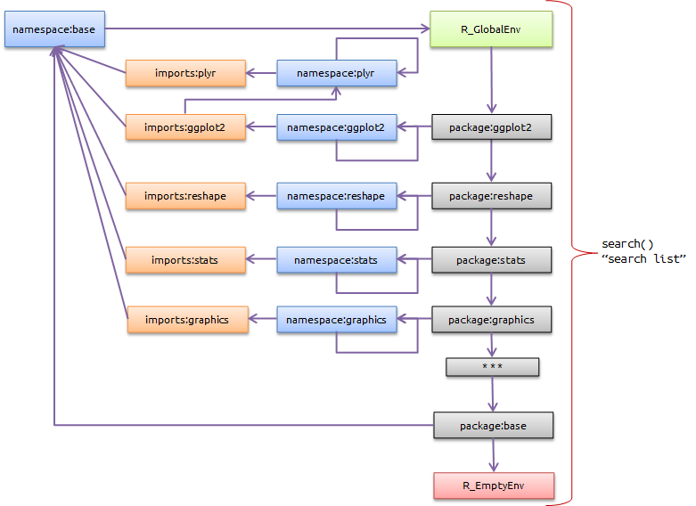
Incidentally, this is another explanation for why there’s no easy way to query an object for the environment that owns it. When we are executing in an environment, we are interested in the objects it owns because we might be looking for one of them. When we find a function we need to know which environment to execute it within. But it's not important in our workflow to identify an arbitrary object’s owning environment.

If your head is spinning then I encourage you to pause and re-read this entire section. Function execution is the most complex piece of the puzzle.

Passing Functions

Feel free to skip this section

It's because functions have an environment property that they can be passed around. Passing a function to another function is a mind-boggling (albeit powerful) feature. I’m not going to explore this too much. At a high level you can think of it as follows. If a function FunctionA( someOtherFunction ) takes another function someOtherFunction as a parameter then FunctionA must have some variability in the way it runs. That variability is governed by the implementation of someOtherFunction. When we construct someOtherFunction, we expect it to run in a particular way. someOtherFunction should have access to the objects in the environment in which it was constructed. That expectation doesn’t change when the function is handed-off to FunctionA . But R creates a new environment for FunctionA. Thankfully that’s not a problem. When someOtherFunction is finally run R looks to the function’s environment property and executes within that environment, not within FunctionA’s environment. So the integrity of our expectation is upheld. In fact, FunctionA can pass someOtherFunction to FunctionB which in turn can pass the function to FunctionC and it has no consequence on how someOtherFunction will run. That’s the magic of a function’s environment property.

That Creepy Caller

The search mechanism does not use the call stack. The call stack is the sequence of function calls that has gotten you to wherever you currently are in the calculation. For example, FunctionA calls FunctionB which in turn calls FunctionC. The call stack just places each of those functions on top of one another in the order in which they were called. Let's say FunctionC needs to execute FunctionD. The wrong way to think about the search mechanism is to follow the callers. That is, if FunctionD is not defined in FunctionC’s executing environment, then look at FunctionB’s executing environment and if not found there then look at FunctionA’s executing environment. The right way to think about the search mechanism is to ask “who owns Function C?” If the owner knows nothing about FunctionD, then maybe the owner’s owner does, and so on.

Unfortunately, the call stack is more intuitive than the chain of enclosing environments. Just remember, whenever R is evaluating a statement the system is simultaneously at the top (or bottom if it’s easier to visualize that way) of two important chains of environments. One is the chain of enclosing environments which is involved in the task of scoping (i.e. where to look next for variable names not found in the frame of the current environment). This is the chain we care about. The other chain is the call stack, which is produced by the sequence of function calls. You can ignore this chain. There are scenarios where it’s necessary to look for a variable via the call stack, but to accomplish that you have to use some special functions in R. Those scenarios are beyond the scope of this article.

A word of caution: R (and some R literature) uses the term “parent” in context of both chains. There’s the function parent.env() which we already know and parent.frame() which is used to interrogate the call stack. This is certainly confusing and it's a historic slip-up. The term “parent” should not be used as a substitute for enclosing environments. It should only be used with the call stack.

Finally, How R searches and finds stuff

So, finally, how does R search and find stuff? R just follows the purple line road in our map above. Let's follow along with an example

Let's say we’re looking for function ggplot. We start at R_GlobalEnv. If ggplot is not in the global environment, then it must be in a package. So R travels down the search list looking for ggplot. This is simply the chain of enclosing environments starting with R_Global. R ultimately find the function in one of the package environments. Although ggplot is found within the package environment, R executes ggplot within the namespace environment as described in the prior section. In this case, we’ve found ggplot in package:ggplot2 and we execute the function within namespace:ggplot2.

Let's say ggplot calls another function MyFunction. A few things can happen:

If MyFunction is defined within ggplot, then we find it immediately since R checks the local environment first. In this case the local environment is the environment created to run ggplot
If not found, then R looks to the enclosing environment of MyFunction’s executing environment which is namespace:ggplot2. If we find MyFunction here, then it’s a case of a package function calling another function in the same package.
If MyFunction is not in the namespace:ggplot2, then R checks the enclosing environment of the namespace environment which is the imports environment. This gives ggplot an opportunity to find MyFunction within a set of explicitly defined package dependencies. This is like ggplot finding a plyr function in our example above.
If MyFunction is not in the imports environment, then we check the enclosing environment of the imports environment which is namespace:base. A base function (i.e. sd() for standard deviation) would be found here and the search would be complete.
If MyFunction is not found in namespace:base, then we are back to the search list. We start by checking R_GlobalEnv. It's unlikely that MyFunction is in R_GlobalEnv. It would be poor practice for a package to expect the user to define some function in the global environment. However, the user could take this as an opportunity to intercept the search by defining her own version of MyFunction in the global environment.
If MyFunction is within a package that’s a dependency of ggplot2 and that dependency is specified in Depends rather than Imports, then the search list is where we would find MyFunction. This is like ggplot looking for a function in the reshape package in our example above. We would hope that no other package has defined the same function and is attached closer to the global environment (as in our reshape2 example above)

All-in-all you just have to determine what the “current” or “local” environment is and following the enclosing environments (the purple arrows) until you find the object you are looking for. Rinse and repeat.

Qualitative Comments

I believe that the search and find mechanism is an adequate design given that R is an interpreted, weakly typed language that supports attaching multiple packages at-will. If we are executing outside of a package (as in R_GlobalEnv) it enables us to find functions inside packages. If we are inside a package it allows the package functions to find the specified dependencies. If we are inside a package or a package’s imports (dependencies), then we have a buffer of base functions before we plunging into the search list. Also, the design ensures that we terminate at R_EmptyEnv if a named object cannot be found, no matter where on the map we are.

All of that said, it's still complicated. When I’m debugging a search-and-find issue it takes a lot of brainpower to figure out what’s going on. Don’t beat yourself up if the same is happening to you.

Skip the search-and-find

If you know exactly which package contains the object desired then you can reference it directly using the :: operator. Simply place the package name before the operator and the name of the object after the operator to retrieve it.

# use :: to get sd
> stats::sd 
function (x, na.rm = FALSE) 
{ 
    ... ( omitted for brevity )
} 
<bytecode: 000000000511D608> 
<environment: namespace:stats>

If the object is not exported or you are unsure, then you can use the ::: operator (notice the extra colon).

# use ::: to get Wilks
> Wilks 
Error: object 'Wilks' not found 
> stats:::Wilks 
function (eig, q, df.res) 
{ 
    ... ( omitted for brevity ) 
} 
<bytecode: 00000000050FE280> 
<environment: namespace:stats>

This operator searches the namespace environment for the given object (as we discussed, non-exported objects do not appear in the package environment, only in the namespace environment). You can validate that by looking at the definition of ::: (remember to include the backticks).

# view the ::: operator function
> `:::` 
function (pkg, name) 
{ 
    pkg <- as.character(substitute(pkg)) 
    name <- as.character(substitute(name)) 
    get(name, envir = asNamespace(pkg), inherits = FALSE) 
} 
<bytecode: 00000000073BAEA8>
<environment: namespace:base>

Thanks

I’d like to thank Josh O’Brien who reviewed a draft version of this post and provided solid feedback. His comments and challenges directly improved the quality of this article. In some cases I lifted text verbatim from his emails (with his permission of course). I am grateful to him for being so generous with his time. I’d also like to thank the R community on StackOverflow for being patient with numerous questions that I’ve posted about topics herein discussed. That community continues to be the absolute best way to get answers about R. Finally, I thank John Chambers for writing the R programmer’s must-have book Software for Data Analysis.

Thoughts?

I welcome your reaction and/or a comment (anonymous or not), below!